---
title: "Adoption, exposure, and the cost of using AI"
subtitle: "A weekly Norwegian vacancy tracker — and why user cost, not capability, shapes what we see"
date: today
date-format: "D. MMMM YYYY"
lang: nb
---
## The empirical object
::: {.callout-note title="Sammendrag"}
Denne siden skiller mellom AI-ens *kapasitet* (eksponering, fra Eloundou m.fl.) og den faktiske *bruken* (adopsjon). Hovedfunnet er at gapet mellom dem først og fremst bestemmes av **brukerkostnaden** ved å ta AI i bruk — ikke av hvor god modellen er. Brukerkostnaden er kostnaden ved å bruke AI trygt og pålitelig: menneskelig tid til å kontrollere og godkjenne resultatet, pluss etterlevelse, personvern og integrasjon. Høy lønn trekker AI inn, mens høy brukerkostnad holder den ute.
I norske stillingsannonser (NAV) er AI fortsatt sjelden nevnt (rundt 1 %) og konsentrert i få yrker. Eksponering forklarer bare svakt hvilke yrker som faktisk etterspør AI; det er **lønnseffekten** som overlever ut-av-utvalg-testing, mens en oppgave-for-oppgave-splitt av brukerkostnaden ennå ikke lar seg identifisere med så tynne data. SSBs egne tall peker samme vei: bruken stiger mens kostnadsbarrieren faller.
Den estimerte **brukerkostnaden** er ikke målt direkte, men et estimat fra en **økonomisk strukturell modell** basert på Lindenlaub og medforfattere (Lindenlaub, Oh, Rodríguez & Veldkamp 2026, «LORV»), der komparative fortrinn — ikke kapasitet alene — avgjør hvilke yrker som tar AI i bruk.
:::
Two numbers get attached to every occupation in the AI-and-jobs debate:
- **Exposure** — how much of the work AI is technically *capable* of doing (Eloundou et al.).
- **Adoption** — how much AI is *actually* being used or asked for.
They are not the same object, and the gap between them is the interesting one. This page
tracks both for the Norwegian labour market — exposure from Statistics Norway (SSB)
occupational data, adoption from a **weekly snapshot of open vacancies** at
[arbeidsplassen.nav.no](https://arbeidsplassen.nav.no) — and argues that what drives the
gap is the **user cost** of putting AI to work.
## Why user cost? A comparative-advantage story
The same 200-year-old logic that governs trade governs this. A firm puts AI on a task only
when AI is **cheaper per unit of output** than the worker — productivity *weighed against
price* — not whenever AI is merely *able*:
$$\underbrace{\frac{Z^{\text{AI}}_k}{r_k}}_{\text{AI's value for money}} \;>\;
\underbrace{\frac{Z^{\text{worker}}_k}{w}}_{\text{the worker's value for money}}$$
The denominator on the left, the **user cost** $r_k$, is the whole story. It is *not* the
price of compute alone — it is the cost of using AI *safely and reliably*: the human time
to **check and sign off** on the output, plus compliance, privacy and integration:
$$r_k \;\approx\; \rho_k \;+\; w\, t^{V}_k .$$
So a task can be highly *exposed* yet barely *adopted* because $r_k$ is high (verification,
accountability, regulation); and high wages $w$ *pull* AI in, because they lower the
worker's value-for-money on the right. **Capability is half the story; the cost of using
AI is the other half** — and it is an organisational and institutional variable, not a
property of the model. This is the central finding of **Lindenlaub, Oh, Rodríguez &
Veldkamp (2026, "LORV")**: across occupations, user cost — not capability — explains most of
*who actually adopts* AI. The exposure measure is from **Eloundou et al. (2024)**, and the
task-chain logic below from **Demirer, Horton, Immorlica & Lucier (2026)**.
### How the cost cascades
The user cost is not fixed. When consecutive tasks are handed to AI, they **chain** — the
interior steps run machine-to-machine and a human verifies only the *end* of the chain. So
verification becomes roughly a **fixed cost per chain, not per step**: as AI grows reliable
and chains lengthen, the cost *per task* falls, and augmentation can tip toward replacement.
{#fig-chain width="100%"}
## What the Norwegian vacancies show
```{python}
#| label: setup
#| code-summary: "Load the latest weekly snapshot + SSB exposure, and merge"
import json, re
import numpy as np
import pandas as pd
import matplotlib.pyplot as plt

KOJA = {"fjord": "#5d79a0", "amber": "#cf9a5c", "mist": "#b1abb0",
        "muted": "#8292ad", "heading": "#e7ecf3"}
plt.rcParams.update({
    "figure.facecolor": "none", "axes.facecolor": "none", "savefig.facecolor": "none",
    "savefig.transparent": True, "text.color": KOJA["mist"], "axes.labelcolor": KOJA["mist"],
    "axes.edgecolor": "#3a4860", "xtick.color": KOJA["muted"], "ytick.color": KOJA["muted"],
    "axes.titlecolor": KOJA["heading"], "axes.grid": True, "grid.color": "#8292ad",
    "grid.alpha": 0.15, "font.size": 11,
})

D = "adoption-tracker/data"
latest = json.load(open(f"{D}/latest.json"))
weekly = pd.read_csv(f"{D}/adoption_weekly.csv")
occ = pd.read_csv(f"{D}/adoption_by_occupation.csv")
occ = occ[occ.date == occ.date.max()].copy()

def norm(s):
    s = str(s).lower().strip().replace("–", "-"); s = re.sub(r"\s+", " ", s)
    return re.sub(r"\s*([/-])\s*", r"\1", re.sub(r"[.;]+$", "", s))

ex = pd.read_csv(f"{D}/exposure_reference.csv")
ex["key"] = ex.occupation_title.map(norm); ex = ex.dropna(subset=["ai_exposure"]).drop_duplicates("key")
occ["key"] = occ.styrk.map(norm)
m = occ.merge(ex[["key", "ai_exposure", "wage_nok_monthly"]], on="key", how="inner")
```
As of the latest snapshot (**`{python} latest['date']`**), `{python} f"{latest['n_ads']:,}"` open
vacancies were collected (of `{python} f"{latest['n_total_open']:,}"` open), of which
**`{python} latest['n_ai']` mention AI (`{python} f"{latest['ai_share']*100:.1f}"`%)**. AI demand
is still rare and concentrated — which is exactly what a high-user-cost world looks like.
```{python}
#| label: fig-adopt-exposure
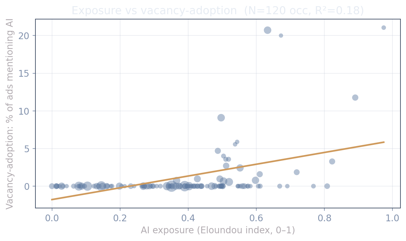
#| fig-cap: "Does exposure predict adoption? Each dot is a Norwegian occupation (≥15 vacancies), sized by vacancy count; vacancy-adoption is the share of its ads mentioning AI. Exposure predicts adoption only weakly — the bulk of the variation is left to user cost."
d = m[m.n_ads >= 15].copy()
x, y, w = d.ai_exposure.values, d.ai_share.values * 100, d.n_ads.values.astype(float)
W = w / w.sum(); xb, yb = np.average(x, weights=W), np.average(y, weights=W)
b1 = np.sum(W * (x - xb) * (y - yb)) / np.sum(W * (x - xb) ** 2); b0 = yb - b1 * xb
r2 = 1 - np.sum(W * (y - (b0 + b1 * x)) ** 2) / np.sum(W * (y - yb) ** 2)

fig, ax = plt.subplots()
ax.scatter(x, y, s=np.sqrt(w) * 7, alpha=.45, color=KOJA["fjord"], edgecolor="none")
xs = np.linspace(x.min(), x.max(), 50); ax.plot(xs, b0 + b1 * xs, color=KOJA["amber"], lw=2)
ax.set_xlabel("AI exposure (Eloundou index, 0–1)")
ax.set_ylabel("Vacancy-adoption: % of ads mentioning AI")
ax.set_title(f"Exposure vs vacancy-adoption  (N={len(d)} occ, R²={r2:.2f})")
plt.tight_layout(); plt.show()
```
The slope is positive but the fit is loose (R² ≈ `{python} f"{r2:.2f}"`): exposure orders
occupations only roughly. In our companion analysis, once capability is controlled the
**wage pull** is the piece that survives out-of-sample testing, while a task-by-task user-cost
split does not — Norway's vacancies are too thin and too uniform in task mix to identify it
yet. That is the case for tracking adoption *over time* and, ultimately, for worker-level data.
## The weekly series (it grows from here)
```{python}
#| label: fig-weekly
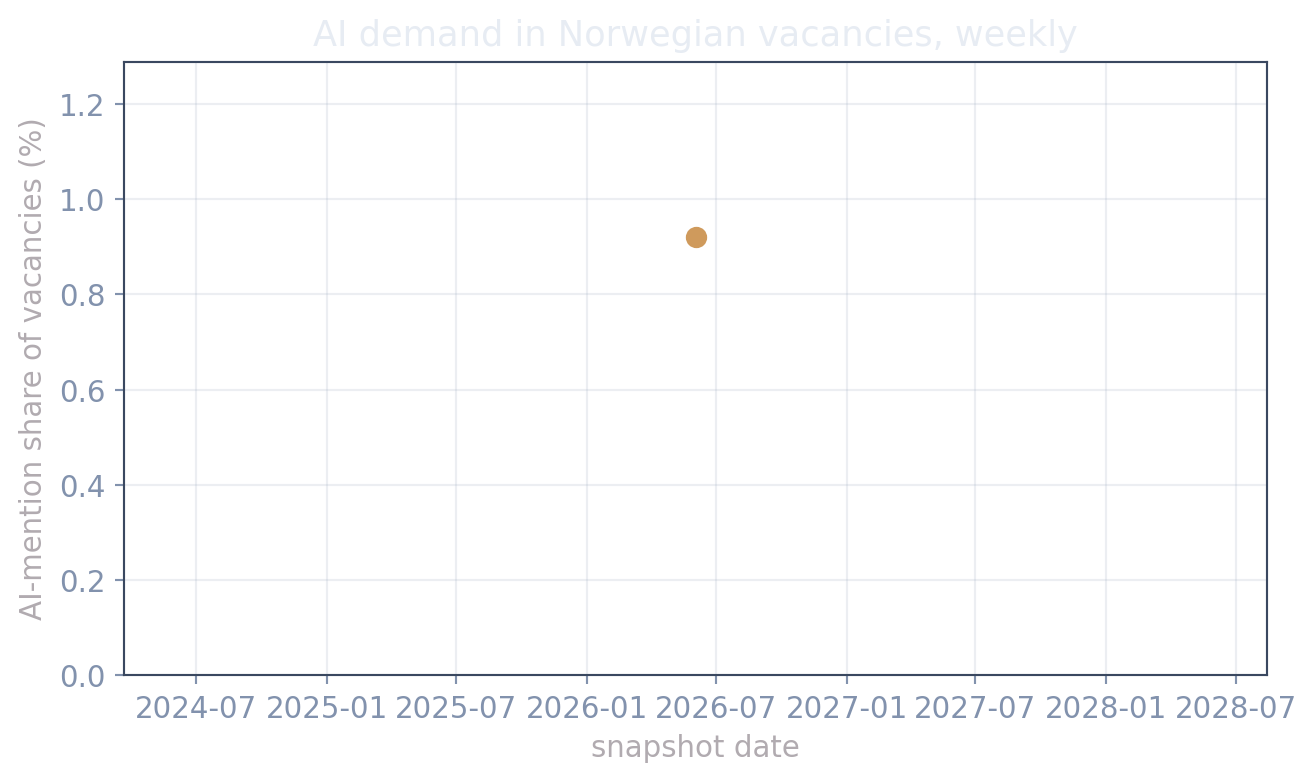
#| fig-cap: "AI-mention share of open Norwegian vacancies, by weekly snapshot. The series starts with this reading and extends every week the collector runs."
wk = weekly.sort_values("date")
fig, ax = plt.subplots()
ax.plot(pd.to_datetime(wk.date), wk.ai_share * 100, "o-", color=KOJA["amber"], lw=1.6, ms=7)
ax.set_ylabel("AI-mention share of vacancies (%)"); ax.set_xlabel("snapshot date")
ax.set_title("AI demand in Norwegian vacancies, weekly")
ax.set_ylim(0, max(1.2, wk.ai_share.max() * 100 * 1.4))
plt.tight_layout(); plt.show()
```
## What firms say: adoption rising, the user cost falling (SSB)
The vacancy signal is demand-side and thin. Statistics Norway's own AI surveys give the
complementary picture — and they say exactly what the comparative-advantage story predicts:
**use is rising while the cost of using AI is the thing holding it back, and that cost is
falling.** (Pulled reproducibly from SSB by `adoption-tracker/`'s rebuild — firm AI-use
table 13265, barriers 13272, individual genAI use 14365.)
```{python}
#| label: fig-ssb-barriers
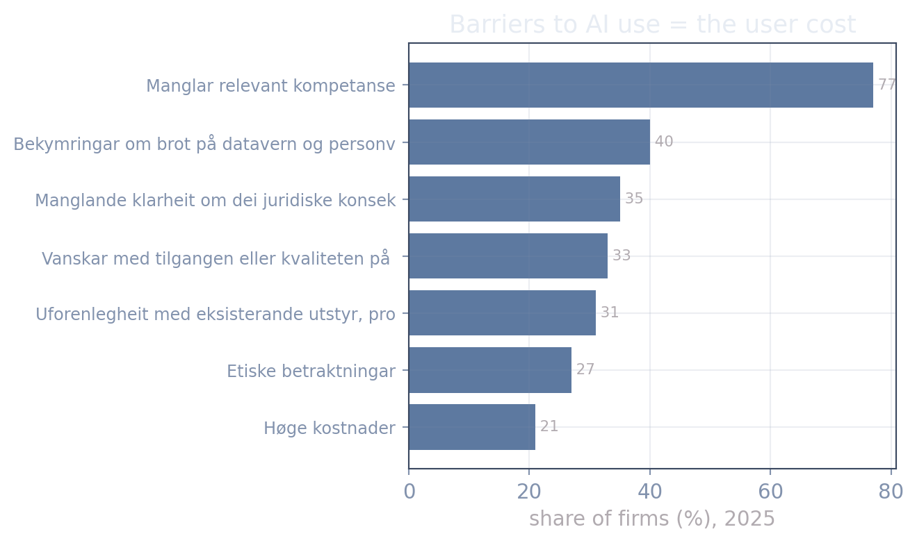
#| fig-cap: "Why Norwegian firms hold back on AI (SSB table 13272, share of firms, latest year). These barriers are the 'user cost' r — and the cost barrier itself has fallen sharply since 2021."
ssb = pd.read_csv("ssb-data/processed/ssb_ai_public_data_focus_extract.csv")
bar = ssb[ssb.table_id == 13272].copy()
yr = bar.Tid_code.max()
b = (bar[bar.Tid_code == yr].sort_values("value").tail(7))
fig, ax = plt.subplots()
ax.barh(range(len(b)), b.value, color=KOJA["fjord"])
ax.set_yticks(range(len(b)))
ax.set_yticklabels([s[:42] for s in b.ContentsCode_label], fontsize=9)
ax.set_xlabel(f"share of firms (%), {yr}")
ax.set_title("Barriers to AI use = the user cost")
for i, v in enumerate(b.value):
    ax.text(v, i, f" {v:.0f}", va="center", fontsize=8, color=KOJA["mist"])
plt.tight_layout(); plt.show()

cost = bar[bar.ContentsCode_label.str.contains("kostnad", case=False, na=False)].sort_values("Tid_code")
use = ssb[(ssb.table_id == 14365) & (ssb.ContentsCode_label.str.contains("Har brukt", na=False))].sort_values("Tid_code")
```
Two trends make the point. The **cost barrier** ("Høge kostnader") fell from
`{python} f"{cost.value.iloc[0]:.0f}"`% (`{python} str(cost.Tid_code.iloc[0])`) to
`{python} f"{cost.value.iloc[-1]:.0f}"`% (`{python} str(cost.Tid_code.iloc[-1])`) — using AI
got cheaper and safer. Over the same window, individual generative-AI use rose from
`{python} f"{use.value.iloc[0]:.0f}"`% to `{python} f"{use.value.iloc[-1]:.0f}"`%. Falling
user cost, rising adoption — the mechanism, in SSB's own numbers.
## Implications: a new occupation inside the chain
Look again at @fig-chain. As tasks chain, the human does not simply disappear from the
interior — they **re-enter at the second-to-last task** (review & edit) as the *in-the-loop
validator*: the person who catches the chain's errors before sign-off. That hybrid
human-+-AI step is a plausible **new occupation**, and where it sits is a policy choice:
- **Lower the user cost and you move the validator earlier and deeper into the chain** —
the AI dividend is unlocked by *training validators and building safe-to-use
infrastructure*, not by waiting for a smarter model.
- It is also the natural **entry point for younger workers** if the new validation work
grows faster than the old rungs disappear — the open empirical question behind
Brynjolfsson, Chandar & Chen (2025).
## Data & method
- **Adoption** — `collect.py` pulls the open vacancies from NAV's public search API once a
week and flags AI with an audited bilingual lexicon (Norwegian + English phrases, brand
names, and uppercase-only abbreviations so "ML" ≠ millilitre). One timestamped snapshot is
archived per run; the share by occupation feeds the figures above.
- **Exposure / employment / wages** — from **Statistics Norway (SSB)**: occupational
employment (table [12542](https://www.ssb.no/en/statbank/table/12542)) and monthly earnings
(table [11418](https://www.ssb.no/en/statbank/table/11418)). `ssb_check.py` runs weekly and
flags when SSB refreshes either table, so the bundled occupational panel can be re-pulled.
::: {.callout-note title="Read these as descriptive, directional facts"}
Vacancy AI-mentions are **demand-side** signals (what employers advertise), not realised
worker use; the snapshot is a recency-capped slice of open postings; mentions are rare
(~1%) and concentrated in a few occupations. So the cross-section orders occupations
loosely and the weekly series is what to watch. The structural "user cost by task" object
needs worker-level / register adoption to identify — this tracker is the first ingredient.
:::
## References
- Lindenlaub, I., Oh, R., Rodríguez, M. A. & Veldkamp, L. (2026). *Beyond Exposure: Predicting AI Adoption Based on Comparative Advantage* ("LORV").
- Demirer, M., Horton, J., Immorlica, N. & Lucier, B. (2026). *Chaining Tasks: AI Automation and the Division of Labor.*
- Eloundou, T., Manning, S., Mishkin, P. & Rock, D. (2024). *GPTs are GPTs: Labor Market Impact Potential of LLMs.*
- Brynjolfsson, E., Chandar, B. & Chen, R. (2025). *Canaries in the Coal Mine: Early Labor-Market Effects of Generative AI.* Stanford Digital Economy Lab.
- Humlum, A. & Vestergaard, E. (2026). *Still Waters, Rapid Currents: Early Labor-Market Transformation under Generative AI.*
- Statistics Norway (SSB), StatBank via PxWebApi v2 — tables 12542, 11418 (occupational employment & earnings) and 13265, 13271, 13272, 14365, 14364 (AI use, purposes, barriers, individual genAI use/non-use).